How short can a proof of impossibility be?

I’m happy to share that my paper “How to Discover Short, Shorter, and the Shortest Proofs of Unsatisfiability” has appeared in the Journal of Artificial Intelligence Research! You can read the full paper here. It is a long one — thirty pages, not counting the proofs of every lemma in the appendices — so in this post, I would like to walk through the ideas behind it without all the machinery.

The short version: when a SAT solver tells you that your formula has no solution, it can also hand you a proof of that claim. We asked how close to the shortest possible those proofs are. The answer, by and large, is: not very close at all.

How to take “no” for an answer

Any algorithm, whether trivial or exquisitely engineered like modern SAT-solving software, expects certain input and produces certain output. To make sense of the paper, it first helps to understand the shape of inputs and especially outputs expected by SAT solvers.

A SAT solver takes a Boolean formula in conjunctive normal form — a big AND of clauses, each clause an OR of literals — and answers whether some assignment of true/false to the variables satisfies all of them at once. When the answer is yes, checking the solver is trivial: it gives you the assignment, and you plug it in.

When the answer is no, there is nothing to plug in. The solver is making a claim about all \(2^n\) assignments, and you surely would not want to take it on faith — solvers are large, heavily optimized programs, and they are used to verify aircraft software and settle open problems in combinatorics. So instead, the solver emits a proof: a written record of the reasoning that led it to the contradiction.

For this paper, the reasoning steps are all instances of a single rule, called resolution. Take two clauses that disagree about exactly one variable. One of them says x, the other says not x. Whichever way x turns out, one of those two literals is false — so everything else in the two clauses has to carry the weight:

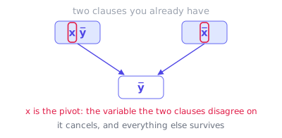
That is the whole rule. It is sound (the conclusion is true whenever the premises are), and it is refutationally complete: if a formula is unsatisfiable, then repeated resolution will eventually derive the empty clause — a clause with no literals left in it, which no assignment can possibly satisfy.

A proof, then, is just a list of clauses: some copied from the input formula, others obtained by resolving two earlier ones, ending with the empty clause. Equivalently — and more usefully for us — it is a directed acyclic graph:

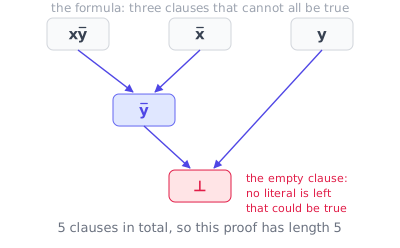
The length of the proof is the number of clauses in it, and the goal of this paper is to minimize that number.

Why the length is worth caring about

Because resolution is not an arbitrary choice of proof system, and it closely mirrors what a CDCL solver actually does. For example, unit propagation — the solver’s workhorse inference — traced backward is a chain of resolution steps. So, a proof is more of an execution trace than the words “certificate” or “proof” would suggest: a short proof corresponds to a run that reached the contradiction in a few steps.

That makes proof length a proxy for a question that is otherwise very hard to ask: how much room for improvement is there, on this particular formula, for this solver? If the solver’s proof is 100 steps and the shortest possible proof is 95, the solver is essentially doing as well as its reasoning system permits, and no amount of heuristic tuning will help. If the shortest proof is 10, something is being left on the table.

This is not a new instinct. The mixed-integer programming community has been asking the same question by computing optimal branch-and-bound trees and comparing them against what solvers actually explore. What was missing on the SAT side was a method that scales far enough to say anything about realistic formulas.

What the community already knew how to do

Proof rewriting applies local transformations — swap two steps, merge a pair of derivations — to a proof you already have. Useful, but by construction local: it cannot restructure large parts of a proof in one move.

Proof trimming (DRAT-trim, LRAT-trim, and friends) walks the proof backward from the empty clause and deletes every step that does not contribute. This works remarkably well because solvers derive an enormous number of clauses that they never end up using. But trimming only removes dead branches from the derivation the solver happened to produce — it never changes the reasoning:

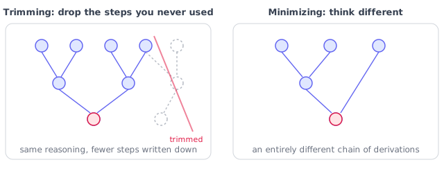
The distinction matters more than it might sound. If the solver wandered into a long, awkward derivation when a short one existed, trimming will faithfully tidy up that long derivation and hand it back to you. It has no way to recover a short reasoning chain that the solver never even started to construct. To do that, you have to stop repairing the trace and start treating proof discovery as an optimization problem in its own right: the feasible set is all valid proofs of this formula, and the objective is length.

That reframing was proposed before us. Mencía and Marques-Silva, and later Peitl and Szeider, built SAT encodings whose satisfying assignments correspond to proofs of a fixed length \(s\); you ask for \(s\), and if the answer is no, you ask for \(s+1\). It is an elegant construction, and it has three problems. It ran out of steam on small formulas, in some evaluations, not even clearing a 12-clause bar. It produces nothing at all until it finishes, so if you run out of time, you have no proof to show for it. And its search space is drowning in symmetry.

The symmetry problem

Symmetry is the interesting one, so let’s look at it properly.

Suppose a proof derives clause \(A\) and clause \(B\), and neither depends on the other. Then “derive \(A\), then \(B\)” and “derive \(B\), then \(A\)” are two different proofs in the sense of being two different lists — but they obviously amount to the same logical argument. A search that enumerates lists will consider both. With many independent derivations, “many” becomes “exponentially many,” and the search spends all of its time essentially rediscovering trains of thought it has already seen.

The standard cure for this condition is to fix some canonical order on the search space; in our problem, one way to put it is as follows: among all clauses eligible at each step, always take the lexicographically smallest. That collapses all the orderings of one DAG into a single representative — a real improvement that was the state-of-the-art approach in this problem, but it does not go far enough, as we discovered.

The issue is that two different DAGs can derive exactly the same set of clauses, but do so through different wiring: for example, clause \(C\) derived from \(A\) and \(B\) in one DAG, and from \(D\) and \(E\) in the other one. Canonical orderings do not touch this, because they only order the steps within a fixed DAG. So the search still visits both, and neither is more informative than the other — just like giving two different solutions to a problem from a math exam does not usually earn you twice the points.

Layer lists

So we changed the representation. Instead of tracking a proof as a sequence, or as a graph, we track it as a sequence of layers, with one strict rule attached.

\(L_0\) is the set of axioms used from the input formula. Each subsequent layer contains clauses obtained by resolving something from the immediately preceding layer with something from any earlier layer. The last layer is just the empty clause. So far this is nothing but a topological ordering of the DAG, drawn in levels.

The difference comes in what we call the take-it-or-leave-it property: every clause must appear in the earliest layer where it could possibly be derived. If a clause follows from the axioms alone, it belongs in \(L_1\) — you are not allowed to postpone it to \(L_2\) and derive it some other way later.

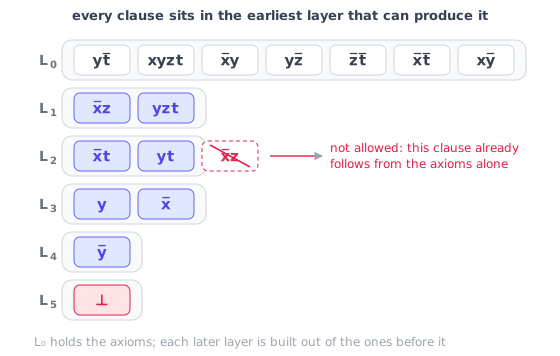
This is a small-sounding condition with a strong consequence, which is Theorem 2 in the paper: for any set of clauses that can be arranged into a proof, there is exactly one layer list containing exactly those clauses. Not “one up to reordering” — one, full stop.

The proof of the theorem is a short induction, and the intuition is that the take-it-or-leave-it rule removes every remaining choice. You have no freedom about when to derive a clause, because “as early as possible” is forced. You have no freedom about how to derive it, because the layer list does not record derivations at all — only which clauses are present. Two proofs on the same clause set are now literally the same object.

Enumerating proofs modulo permutations, therefore, becomes enumerating layer lists, and layer lists can be generated one layer at a time.

Branch-and-bound over proofs

The rest of the algorithm is a fairly conventional branch-and-bound, which is precisely what makes the representation worth the trouble.

A node of the search tree — a subproblem — records four things: the clauses in all layers before the current one, the clauses in the current layer, the clauses committed so far to the next layer, and a set of forgotten clauses. That last one is the bookkeeping that enforces the take-it-or-leave-it property: it records clauses we could have derived and consciously chose not to, so that later layers know not to sneak them in through the back door.

Branching then has to answer: which clauses go in the next layer? Enumerating all subsets is hopeless — the candidate list is quadratic in the clauses derived so far, and its powerset is not something you enumerate. So we build the layer up one candidate at a time. Order the candidates, and split into disjoint cases: take the first one; or give up on the first and take the second; or give up on the first two and take the third; and so on, with a final branch that gives up on all of them and closes the layer.

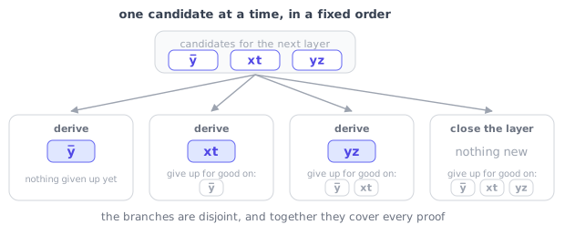
Every proof compatible with the parent lands in exactly one child, which is all a branching rule has to promise. Incidentally, ordering the candidates by descending clause length works markedly better than the reverse — long clauses are weak clauses, they rule out the fewest assignments, and pushing them into the forgotten set early stops the search from wasting effort on them.

Each new subproblem is also handed to a SAT solver, which completes it into some valid (not necessarily short) proof. That gives us an incumbent to prune against from the very first iteration — and it is why the method is anytime: interrupt it somewhere during the run, and you get both a real proof and a real lower bound on the shortest one. That is the direct answer to the second complaint about the encoding approach.

Two ways to prune

Subsumption, or the “frontier.” If your clause set contains both \(x\) and \(x \vee y\), the second one is dead weight: anything you could derive using \(x \vee y\), you could derive at least as well using \(x\), and probably in fewer steps, since \(x\) is the stronger statement. We call the non-subsumed clauses the frontier and branch only on those. Theorem 3 justifies this: any proof with \(m\) steps has a frontier-only counterpart with at most \(m\) steps. As a bonus, if a subproblem is carrying around a non-frontier clause that it can no longer use for anything, the whole subproblem can be discarded.

Counting, for lower bounds. For a minimally unsatisfiable formula — one where dropping any clause makes it satisfiable — every clause must be used, so any proof needs at least \(2\#F - 1\) clauses: the \(\#F\) axioms, plus at least \(\#F - 1\) derivations to combine them. That bound was known. What we needed was a version for the clause sets that show up mid-search, which are not minimally unsatisfiable at all. So we generalized it: look for the smallest minimally unsatisfiable subset of what has been derived so far, and count from there, additionally requiring that subset to contain every clause the subproblem has not yet used for anything.

Finding a smallest unsatisfiable subset is itself hard — \(\Sigma^P_2\)-complete, in fact — so we only ever ask for a lower bound on its size, with a one-second budget. For small inputs, we run a second, tiny branch-and-bound, and its bounding rule is a nice piece of counting that is worth spelling out. A clause with three literals is falsified by exactly one assignment in eight: fix its three literals to the wrong values, and the remaining variables are free. So a set of \(k\) three-literal clauses can rule out at most \(k/8\) of all assignments. An unsatisfiable formula has to rule out all of them:

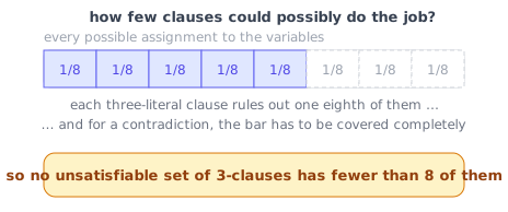
Generalize that to mixed clause lengths — a clause with \(w\) literals covers \(2^{-w}\) of the space — and you get a lower bound you can evaluate by sorting the clauses and adding up fractions until they reach 1.

Does it work?

This time, we get two questions for the price of one, because the method wears two hats: as an exact algorithm that proves optimality, and as an anytime heuristic that just tries to find something short.

As an exact method, on the small synthetic formulas where optimality is reachable at all, we solve roughly twice as many instances as the encoding approach — 428 additional minimally unsatisfiable instances on top of the 396 both approaches manage, and exactly one instance that the baseline solves and we do not. In the instances both handle, we are typically faster by orders of magnitude; the only cases where we lose are ones where both approaches finish in under ten seconds anyway.

The runtime scales exponentially in something we can name, which I find even more interesting than the speedup itself: the gap between the true shortest proof and that \(2\#F - 1\) lower bound. When the gap is zero, the search stops the moment it stumbles on an optimal proof, and the time barely depends on formula size at all. When the gap is nonzero, every subproblem sharing the root’s bound has to be exhausted before optimality can be declared — and that is where the time goes.

As an anytime method, we ran it against CaDiCaL on the 878 unsatisfiable formulas from every SAT Competition between 2002 and 2025 that CaDiCaL refutes within fifteen seconds, comparing against its proofs after trimming. The typical reduction is 15–50%. On the synthetic families, it is 25–50%, with subset-cardinality formulas reliably above 40%.

Typical figures are important, but tails are perhaps even more interesting:

• Formulas known to be hard for resolution — Tseitin formulas and relatives — see consistent two- to nine-fold reductions.
• Proof for planning formulas (at the median) halve. The single largest reduction we saw was on a multi-robot path planning formula, where the trimmed solver proof has over four million resolution steps, and the proof we found has fewer than twenty-five thousand. That is a factor of 163.
• Verification formulas, on the other hand, behave like the dataset average. Whatever happens in planning encodings stays in the planning domain.

And one result I did not expect: proofs that trim well almost never shrink further, and proofs that shrink well almost never trim well. Across the whole benchmark set, there are only five formulas where trimming gave a five-fold reduction and our method then gave another five-fold reduction on top. The two techniques are attacking genuinely different kinds of waste — trimming removes work the solver did and didn’t need; we replace the work it did with different work.

What this does not show

The paper has a section on limitations, and I think it will not hurt to repeat it here, since the promise of solving the proof minimization problem is so large:

Resolution is not modern SAT solving. It models CDCL without inprocessing, which is a real solver from about two decades ago. Contemporary solvers use inferences that resolution cannot simulate efficiently: symmetry breaking, pseudo-Boolean reasoning, Gaussian elimination, and decision diagrams. Pigeonhole formulas are the canonical embarrassment — trivial to refute with a counting argument on paper, provably exponential in resolution.

Even the proof format is an approximation. CDCL is more faithfully modeled by RUP than by resolution; minimizing resolution steps minimizes propagations, whereas what you would really like to minimize is conflict clauses. The two systems are polynomially related, which is enough for asymptotics and awkward for measurement.

Existence of short proofs does not imply short proofs are findable. Resolution is not automatizable under plausible complexity assumptions. So even where we demonstrate that a formula family admits proofs far shorter than a solver produces, that is not a recipe for a solver that finds them.

And it is memory-hungry. Best-first search over subproblems that each carry clause sets around is exactly as expensive as it sounds; on one pigeonhole instance, we ran out of 16 GB while solving both smaller and larger ones.

Where this goes

For all the limitations of this work, I think the headline result stands on its own. Solver proofs are not merely padded with unused steps — trimming already told us that. They are often structurally far from optimal, sometimes by two orders of magnitude, and the shorter proof is not a tidied-up version of the long one. It is a different argument entirely. Of course, I think it would be interesting to see how to run this argument in richer proof systems — and use it to inform the design of new solver components.

Thanks for reading!